Use of Take Formula.
Take formula is used for data retrieval by given rows and columns that’s we want to take.
In other words, Return a specified numbers of contiguous rows and columns from the start or end of the array.
Syntax.
=TAKE(array, rows,[columns])
The TAKE function syntax has the following arguments:
- array: The array from which to take rows or columns.
- rows: The number of rows to take. A negative value takes from the end of the array.
- columns: The number of columns to take. A negative value takes from the end of the array.
Errors.
- Excel returns a #CALC! error to indicate an empty array when either rows or columns is 0.
- Excel returns a #NUM when array is too large.
Let’s see an Example 1.
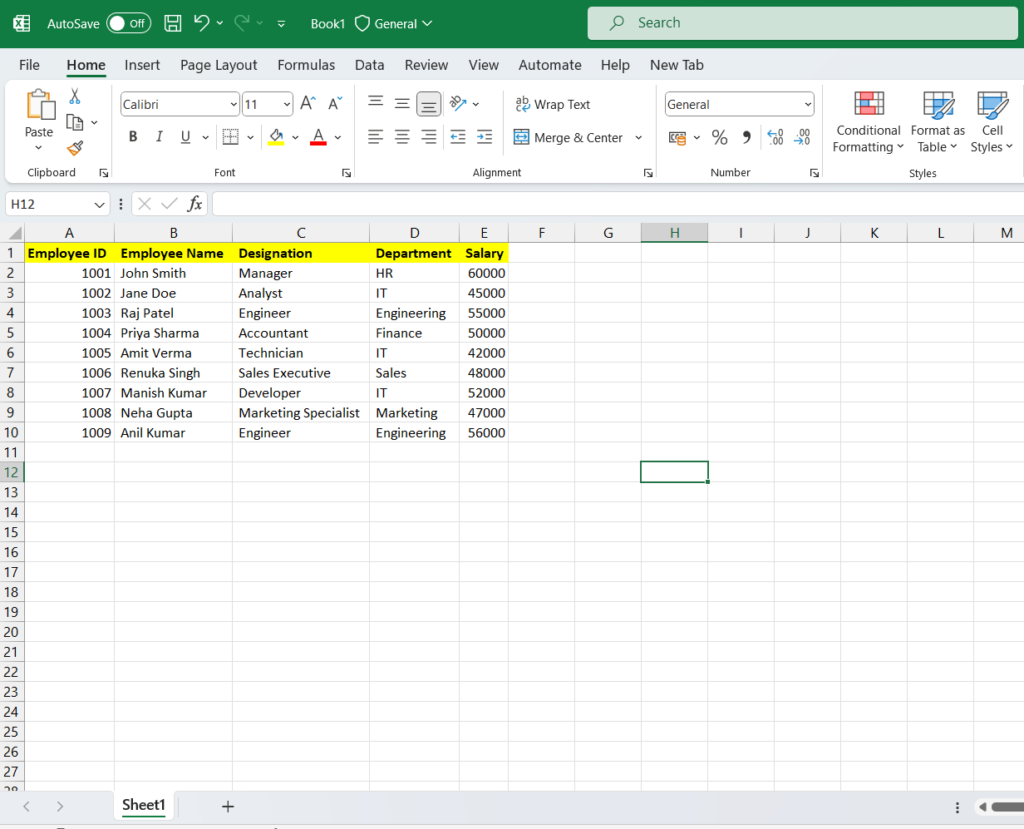
Here we have some data in Excel. You can download it from CLICK HERE

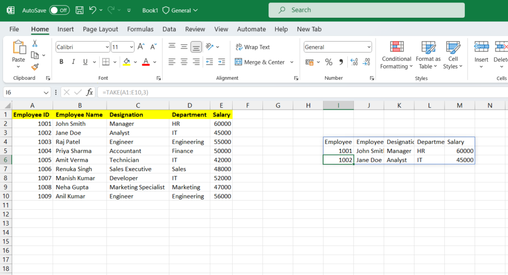
Returns the first three rows from the array in range A1:E10.
Formulas.
=TAKE(A1:E10,3) like see in the figure.

Result is…..

Example 2:
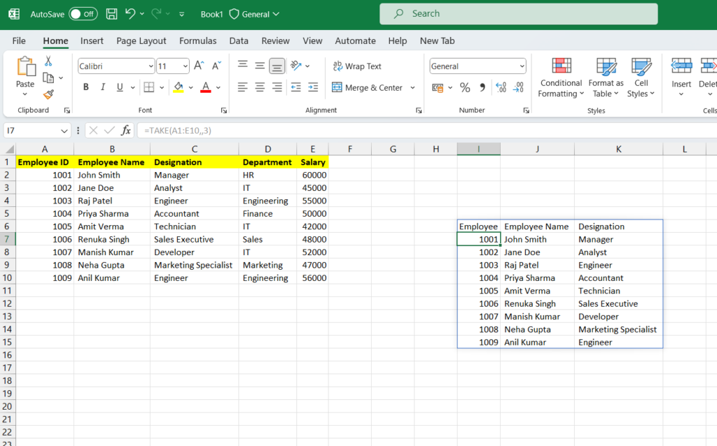
Returns the first three columns from the array in range A1:E10.
Formulas.
=TAKE(A1:E10,,3) and result will be there like in the figure.

Example 3:
Returns the last three rows from the array in range A1:E10.
Formulas.
=TAKE(A1:E10,-3) and result will be there like in the figure.

Example 4:
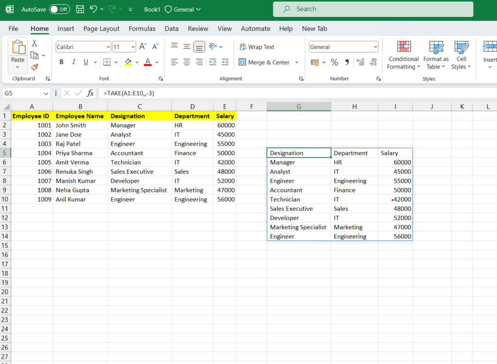
Returns the last three columns from the array in range A1:E10.
Formulas.
=TAKE(A1:E10,,-3) and result will be there like in the figure.

Example 5:
Returns the first three rows and first two columns from the array in range A1:E10.
Formulas.
=TAKE(A1:E10,3,2) and result will be there like in the figure.

